Day 3: Variant Analysis in R

Introduction

Now that we have annotated our somatic variants with VEP, we can move from command-line annotation to R-based analysis and visualization. In this section, we will load VEP output into R, explore the distribution of variant consequences, and create informative visualizations to help prioritize variants of interest.

Setup

Switch to RStudio

For the R exercises, open RStudio in your browser. Use the same IP address as your VS Code environment, but change the port: replace 9xxx with 10xxx (e.g., if your VS Code is at http://12.345.678.91:9001, RStudio is at http://12.345.678.91:10001). Log in with username rstudio and the password provided.

First, we load the VEP annotated output into R and extract some useful fields from the Extra column. Copy and run this setup code in your RStudio console:

Setup code

# get libraries
library(readr)
library(ggplot2)
library(dplyr)
library(tidyr)
library(stringr)

# VEP output in
vep_data <- read_tsv(
  "variants/chr6ch17_mutect2_annotated_with_clinVar.txt",
  comment = "##"
)

# better to set up a ggplot2 theme
theme_course <- function() {
  theme_minimal(base_size = 14) +
    theme(
      plot.title = element_text(size = 16, face = "bold"),
      axis.title = element_text(size = 14, face = "bold"),
      axis.text = element_text(size = 12),
      legend.title = element_text(size = 13, face = "bold"),
      legend.text = element_text(size = 12),
      strip.text = element_text(size = 13, face = "bold"),
      legend.position = "bottom"
    )
}

# Split when it contains multiple values
consequences_df <- vep_data |>
  separate_rows(Consequence, sep = "&") |>
  select(Consequence)

# get chr
vep_data <- vep_data |>
  separate_wider_delim(Location, delim = ":", names = c("chr", "position")) |>
  mutate(chr = factor(chr, levels = c("chr6", "chr17")))

# Extract IMPACT from Extra column
vep_data$IMPACT <- gsub(".*IMPACT=([^;]+).*", "\\1", vep_data$Extra)

# get nice data out of the df
extract_field <- function(data, field) {
  gsub(paste0(".*", field, "=([^;]+).*"), "\\1", data$Extra)
}

# combine multiple fields
vep_data <- vep_data |>
  mutate(
    IMPACT = extract_field(pick(everything()), "IMPACT"),
    SYMBOL = extract_field(pick(everything()), "SYMBOL"),
    VARIANT_CLASS = extract_field(pick(everything()), "VARIANT_CLASS"),
    BIOTYPE = extract_field(pick(everything()), "BIOTYPE")
  )

Exercise 5

Visualize the data from VEP

Objective: Learn how to quickly visualize your variants.

Task: Visualize:

Consequence plot, to visualize the distribution of consequences?
Consequence plot, by chromosome?
Can we see the consequence colored by impact?
Can we see the consequence colored by impact by chromosome?
What are the most common variant classes?
What are the most common biotypes?
Bonus: ClinVar, SIFT, and PolyPhen
Bonus: Gene level damage

1. Consequence plot, to visualize the distribution of consequences

# consequence plot
ggplot(vep_data, aes(x = reorder(Consequence, table(Consequence)[Consequence]))) +
  geom_bar() +
  coord_flip() +
  theme_minimal() +
  labs(title = "Distribution of \n Variant Consequences",
       x = "Consequence Type",
       y = "Count") +
  theme_course()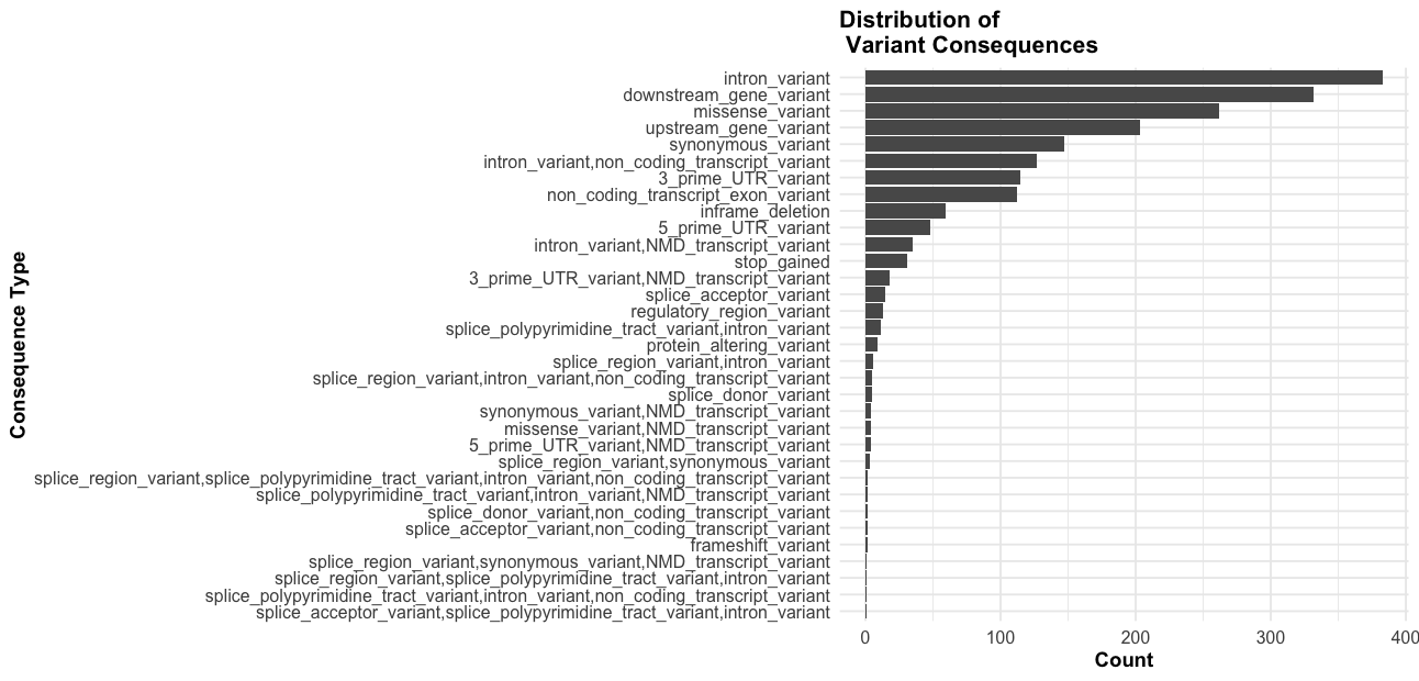

2. Consequence plot, by chromosome

# consequence plot
ggplot(vep_data, aes(x = reorder(Consequence, table(Consequence)[Consequence]))) +
  geom_bar() +
  coord_flip() +
  theme_minimal() +
  labs(title = "Distribution of \n Variant Consequences",
       x = "Consequence Type",
       y = "Count") +
  facet_grid(~chr) +
  theme(
    legend.position = "bottom"
  ) +
  theme_course()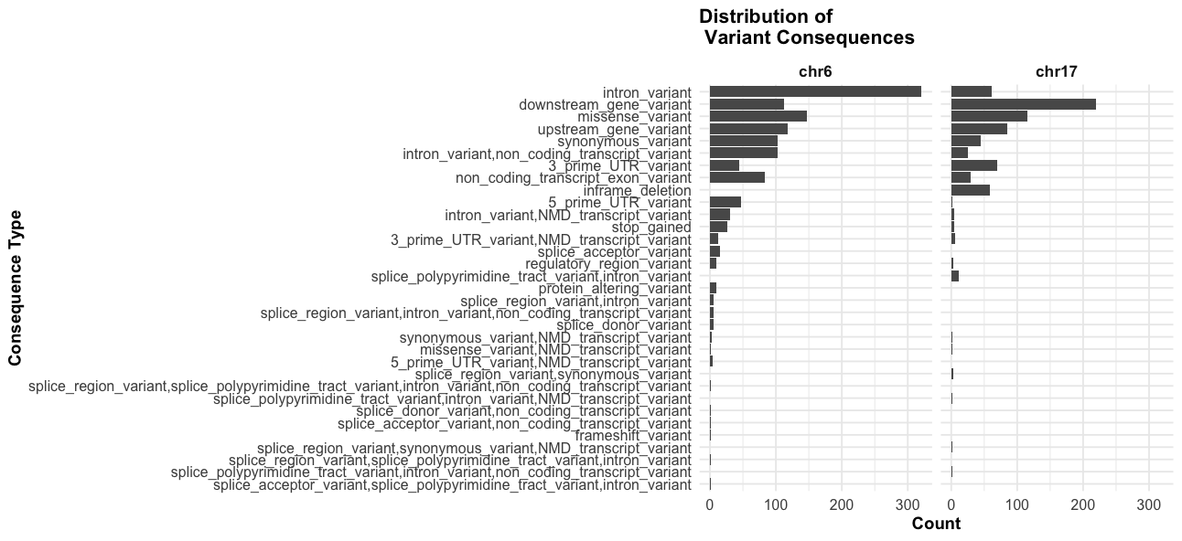

3. Can we see the consequence colored by impact

# Impact + Consequence plot
ggplot(vep_data, aes(x = reorder(Consequence, table(Consequence)[Consequence]), fill = IMPACT)) +
  geom_bar() +
  coord_flip() +
  theme_minimal() +
  scale_fill_brewer(palette = "Set1") +
  labs(title = "Variant Consequences \n by Impact",
       x = "Consequence Type",
       y = "Count") +
  theme(
    legend.position = "bottom"
  ) +
  theme_course()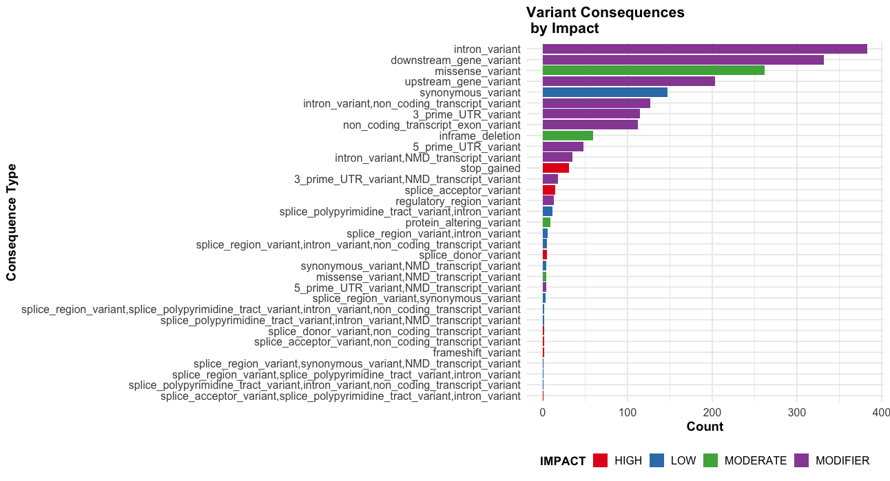

4. Can we see the consequence colored by impact by chromosome

# Impact + consequence plot x chr
ggplot(vep_data, aes(x = reorder(Consequence, table(Consequence)[Consequence]), fill = IMPACT)) +
  geom_bar() +
  coord_flip() +
  theme_minimal() +
  scale_fill_brewer(palette = "Set1") +
  labs(title = "Variant Consequences \n by Impact",
       x = "Consequence Type",
       y = "Count") +
  facet_grid(~chr) +
  theme(
    legend.position = "bottom"
  ) +
  theme_course()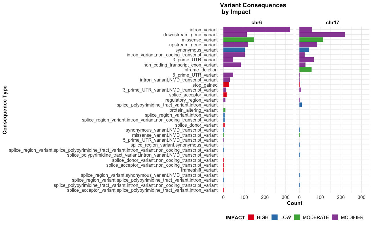

5. What are the most common variant classes?

# variant class plot
vep_data |>
  count(VARIANT_CLASS) |>
  arrange(desc(n)) |>
  ggplot(aes(x = reorder(VARIANT_CLASS, n), y = n)) +
  geom_bar(stat = "identity", fill = "steelblue") +
  coord_flip() +
  theme_minimal() +
  labs(title = "Distribution of \n Variant Classes",
       x = "Variant Class",
       y = "Count"
       ) +
  theme_course()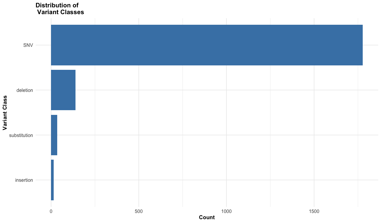

6. What are the most common biotypes?

# biotype distribution
ggplot(vep_data, aes(x = reorder(BIOTYPE, table(BIOTYPE)[BIOTYPE]))) +
  geom_bar(fill = "steelblue") +
  coord_flip() +
  theme_minimal() +
  labs(title = "Distribution of \n Biotypes",
       x = "Biotype",
       y = "Count"
       ) +
  theme_course()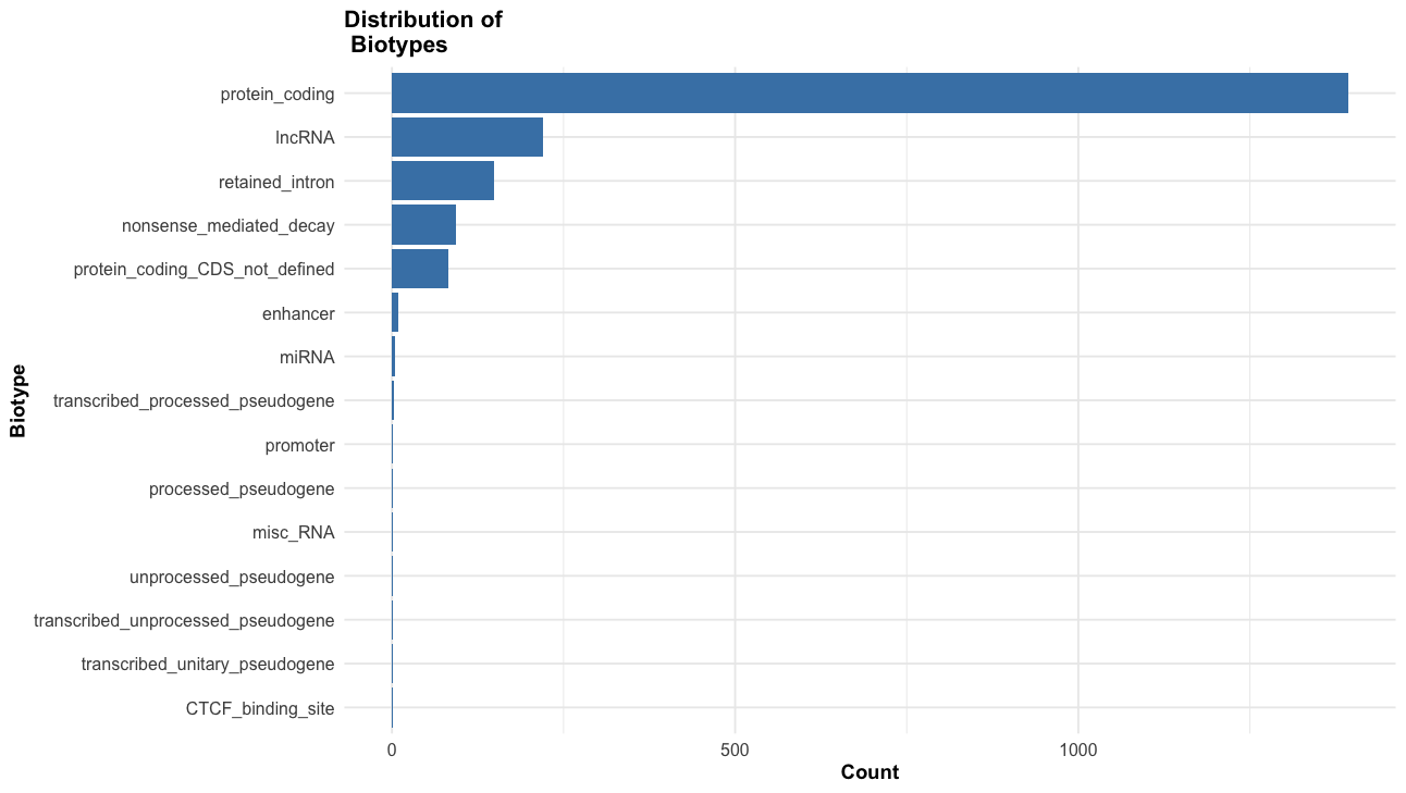

7. Bonus: ClinVar, SIFT, and PolyPhen

# Extract SIFT
vep_data$sift <- str_extract(vep_data$Extra, "SIFT=.*?;")
vep_data$sift <- str_replace(vep_data$sift, "SIFT=", "")
vep_data$sift <- str_replace(vep_data$sift, ";", "")
vep_data$sift <- str_replace(vep_data$sift, "\\(.*\\)", "")

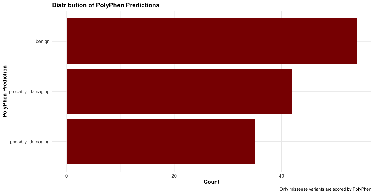
# Extract PolyPhen
vep_data$polyphen <- vep_data$Extra |>
  str_extract("PolyPhen=.*?;") |>
  str_replace("PolyPhen=", "") |>
  str_replace(";", "") |>
  str_replace("\\(.*\\)", "")

# Extract ClinVar
vep_data$clinvar <- vep_data$Extra |>
  str_extract("ClinVar_CLNSIG=.*?;") |>
  str_replace("ClinVar_CLNSIG=", "") |>
  str_replace(";", "")

# Distribution of SIFT predictions
ggplot(subset(vep_data, !is.na(sift)),
       aes(x = reorder(sift, table(sift)[sift]))) +
  geom_bar(fill = "steelblue") +
  coord_flip() +
  theme_minimal() +
  labs(title = "Distribution of SIFT Predictions",
       x = "SIFT Prediction",
       y = "Count",
       caption = "Only missense variants are scored by SIFT") +
  theme_course()

# Distribution of PolyPhen predictions
ggplot(subset(vep_data, !is.na(polyphen)),
       aes(x = reorder(polyphen, table(polyphen)[polyphen]))) +
  geom_bar(fill = "darkred") +
  coord_flip() +
  theme_minimal() +
  labs(title = "Distribution of PolyPhen Predictions",
       x = "PolyPhen Prediction",
       y = "Count",
       caption = "Only missense variants are scored by PolyPhen") +
  theme_course()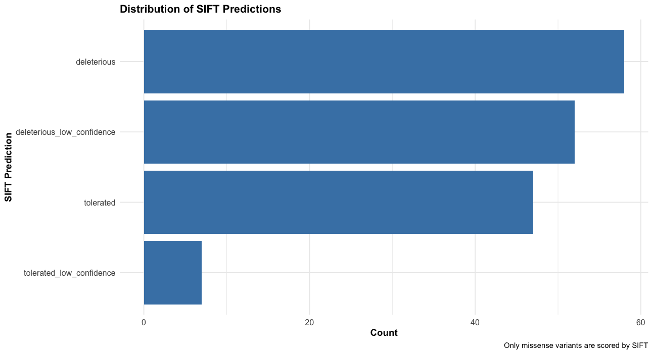

Combined SIFT and PolyPhen predictions with Impact

# Only for variants with both predictions
p3 <- subset(vep_data, !is.na(sift) & !is.na(polyphen)) |>
  ggplot(aes(x = sift, fill = IMPACT)) +
  geom_bar() +
  facet_wrap(~polyphen) +
  coord_flip() +
  theme_minimal() +
  scale_fill_brewer(palette = "Set1") +
  labs(title = "SIFT and PolyPhen Predictions by Impact",
       x = "SIFT Prediction",
       y = "Count") +
  theme(legend.position = "bottom") +
  theme_course()

# 4. ClinVar significance with impact
p4 <- subset(vep_data, !is.na(clinvar)) |>
  ggplot(aes(x = reorder(clinvar, table(clinvar)[clinvar]), fill = IMPACT)) +
  geom_bar() +
  coord_flip() +
  scale_fill_brewer(palette = "Set1") +
  theme_minimal() +
  labs(title = "Clinical Significance by Impact",
       x = "ClinVar Clinical Significance",
       y = "Count") +
  theme(legend.position = "bottom") +
  theme_course()

# 5. For missense variants only - comparison of predictions
p5 <- subset(vep_data, Consequence == "missense_variant" & !is.na(sift) & !is.na(polyphen)) |>
  ggplot(aes(x = sift, fill = polyphen)) +
  geom_bar(position = "dodge") +
  theme_minimal() +
  scale_fill_brewer(palette = "Set2") +
  labs(title = "SIFT vs PolyPhen Predictions\nfor Missense Variants",
       x = "SIFT Prediction",
       y = "Count",
       fill = "PolyPhen Prediction") +
  theme(axis.text.x = element_text(angle = 45, hjust = 1)) +
  theme_course()

Plots

print(p3)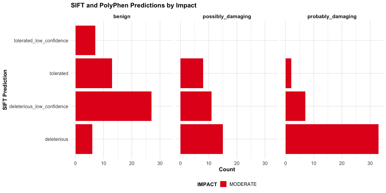

print(p4)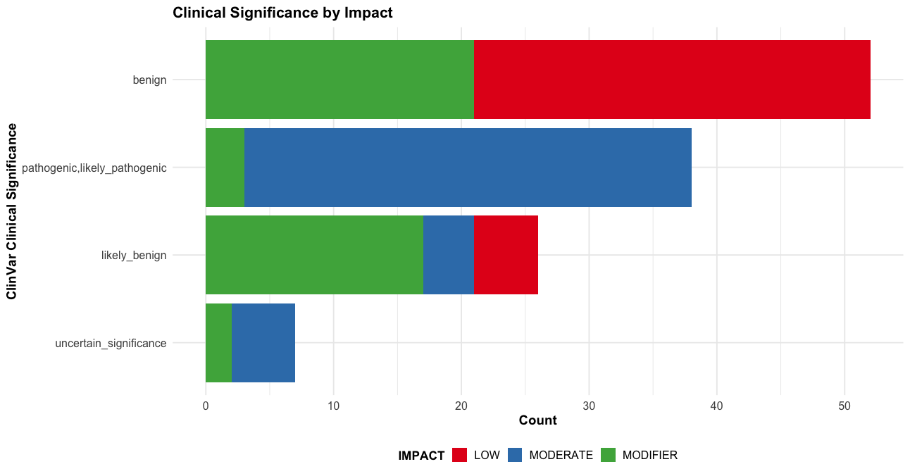

print(p5)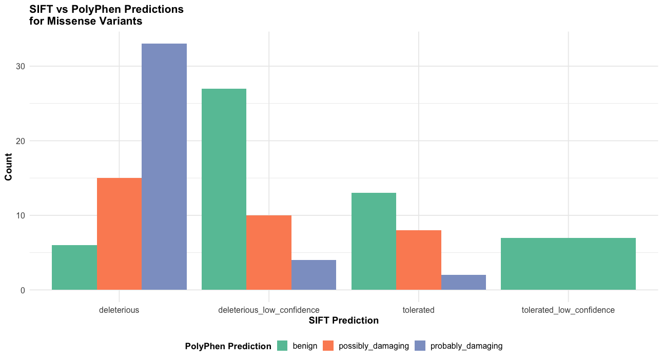

8. Bonus: Gene level damage

# Gene-level summary - most frequently mutated genes
p6 <- vep_data |>
  filter(!is.na(SYMBOL) & SYMBOL != "") |>
  count(SYMBOL, chr) |>
  arrange(desc(n)) |>
  slice_head(n = 20) |>
  ggplot(aes(x = reorder(SYMBOL, n), y = n, fill = chr)) +
  geom_col() +
  coord_flip() +
  scale_fill_brewer(palette = "Set1") +
  labs(title = "Top 20 Most Frequently Mutated Genes",
       x = "Gene Symbol",
       y = "Number of Variants",
       fill = "Chromosome") +
  theme_course()

# High impact variants by gene
p7 <- vep_data |>
  filter(IMPACT %in% c("HIGH", "MODERATE") & !is.na(SYMBOL) & SYMBOL != "") |>
  count(SYMBOL, IMPACT) |>
  arrange(desc(n)) |>
  slice_head(n = 30) |>
  ggplot(aes(x = reorder(SYMBOL, n), y = n, fill = IMPACT)) +
  geom_col() +
  coord_flip() +
  scale_fill_manual(values = c("HIGH" = "#d62728", "MODERATE" = "#ff7f0e")) +
  labs(title = "Genes with High/Moderate Impact Variants",
       x = "Gene Symbol",
       y = "Number of Variants",
       fill = "Impact Level") +
  theme_course()

Plots

print(p6)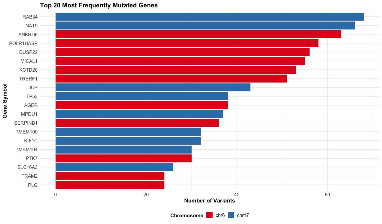

print(p7)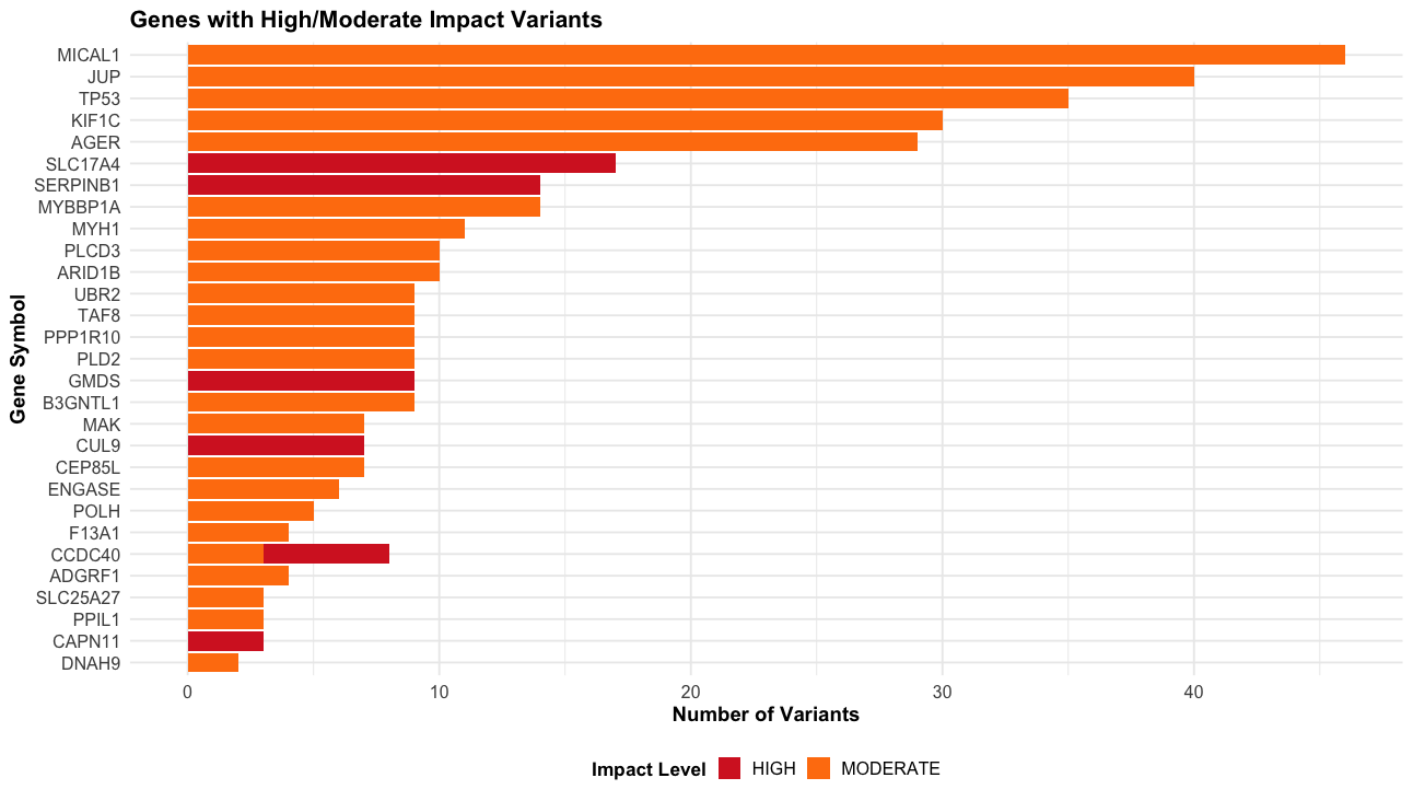

VEP Performance Optimization

For large-scale analyses, consider these optimization strategies:

Using Cache:

--cache
--dir_cache /path/to/cache
--offline

Parallel Processing:

--fork 4

Minimal Output:

--fields "Consequence,IMPACT,SYMBOL,Feature"
--no_stats

Tips for Cancer Variant Analysis

Quality Control
- Filter low-quality variants before VEP annotation
- Use matched normal samples when available (if not consider PONs)
- Consider sequencing artifacts
Annotation Strategy
- Use multiple prediction algorithms
- Consider tissue-specific expression
- Include population frequencies
- Add clinical annotations
Interpretation Guidelines
- Use cancer-specific frameworks for somatic variants
- Document all filtering criteria
- Maintain version control of annotation sources

Databases

COSMIC: https://cancer.sanger.ac.uk/cosmic
ClinVar: https://www.ncbi.nlm.nih.gov/clinvar/
gnomAD: https://gnomad.broadinstitute.org/
ALFA 4: https://www.ncbi.nlm.nih.gov/snp/docs/gsr/alfa/ALFA_20250407153717/
OncoKB: https://www.oncokb.org/

Download data to COSMIC

For COSMIC: We cannot provide those files (they require licensing), you need to register and download the files. CosmicMutantExport.tsv.gz You can register here:

Best Practices from Literature

Key Recommendations

From McLaren et al. (2016) - VEP Paper:

Use --pick or --per_gene to manage transcript complexity
Combine multiple prediction algorithms for consensus
Always document VEP version and cache version for reproducibility

For Cancer Analysis:

Filter common variants (gnomAD MAF < 0.001, i.e., 0.1%) for somatic analysis — variants above this frequency are almost certainly germline
Consider tissue-specific expression data when available
Use multiple evidence sources (ClinVar + COSMIC + literature)
Validate high-priority variants with orthogonal methods

Tools and Documentation

VEP Documentation: http://www.ensembl.org/info/docs/tools/vep/
VEP GitHub: https://github.com/Ensembl/ensembl-vep
Cancer Gene Census: https://cancer.sanger.ac.uk/census

Remember to:

Always verify file paths and permissions
Check input data format and quality
Validate output at each step
Consider computational resources when processing large datasets
Document any modifications to the pipeline

Quick Reference

VEP Command Cheatsheet

Basic annotation:

vep -i input.vcf \
    --cache ${HOME}/project/data/.vep \
    --offline \
    --assembly GRCh38 \
    -o output.txt

With common options:

vep -i input.vcf \
    --cache ${HOME}/project/data/.vep \
    --offline \
    --assembly GRCh38 \
    --everything \
    --fork 2 \
    --vcf \
    -o output.vcf

Filter high-impact:

filter_vep -i input.txt \
    -o filtered.txt \
    --filter "IMPACT is HIGH or IMPACT is MODERATE"

Output format options:

# VEP default format (custom tab-delimited, suitable for filter_vep)
vep ... -o output.txt
# Explicit tab format with header (better for loading into R/pandas)
vep ... --tab -o output.txt

# VCF output (standard variant format)
vep ... --vcf -o output.vcf

# Compressed VCF (saves space, ready for tabix)
vep ... --vcf --compress_output bgzip -o output.vcf.gz

# Custom tab-delimited fields (choose specific columns)
vep ... --tab --fields "Location,Allele,Gene,SYMBOL,Consequence,IMPACT,SIFT,PolyPhen" \
    -o custom_output.txt

Common flags:

--pick: One consequence per variant
--per_gene: One consequence per gene
--fork N: Use N CPU cores
--no_stats: Skip HTML summary (faster)
--tab: Explicitly requests tab-separated output with a header line suitable for downstream tools (R, pandas)
--vcf: VCF format output
--json: Outputs to JSON format
--fields: Choose specific output columns

References

McLaren W, et al. The Ensembl Variant Effect Predictor. Genome Biology (2016)
Eilbeck K, et al. The Sequence Ontology: a tool for the unification of genome annotations. Genome Biology (2005)
Richards S, et al. Standards and guidelines for the interpretation of sequence variants. Genetics in Medicine (2015)
Terry A. Brown, et al. Genomes 5 (2023)