Variant Allele Frequency (VAF) Analysis

Why VAF matters

As we saw in the lectures, the Variant Allele Frequency (VAF) (the fraction of reads supporting the alternate allele) is central to somatic variant interpretation. It reflects tumor purity, clonality, and copy number state:

• A clonal heterozygous variant in a pure tumor → VAF ≈ 50%
• Lower tumor purity reduces observed VAF proportionally
• Subclonal variants (present in only a fraction of tumor cells) → low VAF
• Copy number alterations shift expected VAF away from simple ratios

Understanding the VAF distribution of your variant calls helps you assess sample quality, estimate clonality, and distinguish driver mutations from passenger noise.

Extract VAF from the Mutect2 VCF

The tumor VAF is stored in the Mutect2 VCF’s FORMAT/AF field. This information is not carried over into VEP text output, so we extract it directly from the filtered VCF using bcftools query.

ImportantPrepare the VAF data

Run this command in the terminal to create a simple table R can read:

bcftools query \
  -s tumor \
  -f '%CHROM\t%POS\t%REF\t%ALT\t[%AF]\n' \
  ~/project/variants/somatic.filtered.PASS.vcf.gz \
  > ~/project/variants/vaf_data.tsv

The -s tumor flag extracts data only for the tumor sample. This gives us chromosome, position, reference allele, alternate allele, and the tumor allele frequency (one variant per line, no VCF complexity).

VAF Analysis in R

ImportantSwitch to RStudio

For the R exercises, open RStudio in your browser. Use the same IP address as your VS Code environment, but change the port: replace 9xxx with 10xxx (e.g., if your VS Code is at http://12.345.678.91:9001, RStudio is at http://12.345.678.91:10001). Log in with username rstudio and the password provided.

First, load the required libraries and read in the VAF data we just extracted. Copy and run this setup code in your RStudio console:

NoteSetup code (from TSV format)

library(readr)
library(ggplot2)
library(dplyr)

# Course theme
theme_course <- function() {
  theme_minimal(base_size = 14) +
    theme(
      plot.title = element_text(size = 16, face = "bold"),
      axis.title = element_text(size = 14, face = "bold"),
      axis.text = element_text(size = 12),
      legend.title = element_text(size = 13, face = "bold"),
      legend.text = element_text(size = 12),
      strip.text = element_text(size = 13, face = "bold"),
      legend.position = "bottom"
    )
}

# Load VAF data
vaf_data <- read_tsv(
  "variants/vaf_data.tsv",
  col_names = c("chr", "pos", "ref", "alt", "tumor_af"),
  col_types = "ciccd"
) |>
  mutate(chr = factor(chr, levels = c("chr6", "chr17")))

Exercises

ImportantVisualize the VAF distribution

Task: Create the following visualizations:

1. Histogram of tumor VAF — what does the distribution look like?
2. VAF distribution by chromosome — do chr6 and chr17 differ?
3. Density plot — can you identify clonal vs subclonal peaks?

Think about: Based on the lectures, what would a VAF of ~50% suggest? What about variants with VAF < 10%?

Tip1. VAF histogram

ggplot(vaf_data, aes(x = tumor_af)) +
  geom_histogram(binwidth = 0.05, fill = "steelblue", color = "white") +
  labs(
    title = "Distribution of Tumor Variant Allele Frequencies",
    x = "Variant Allele Frequency (VAF)",
    y = "Count"
  ) +
  scale_x_continuous(labels = scales::percent_format(), limits = c(0, 1)) +
  theme_course()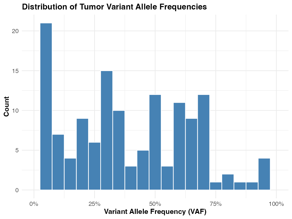

Tip2. VAF by chromosome

ggplot(vaf_data, aes(x = tumor_af, fill = chr)) +
  geom_histogram(binwidth = 0.05, color = "white", alpha = 0.7, position = "identity") +
  labs(
    title = "VAF Distribution by Chromosome",
    x = "Variant Allele Frequency (VAF)",
    y = "Count",
    fill = "Chromosome"
  ) +
  scale_x_continuous(labels = scales::percent_format(), limits = c(0, 1)) +
  scale_fill_brewer(palette = "Set1") +
  theme_course()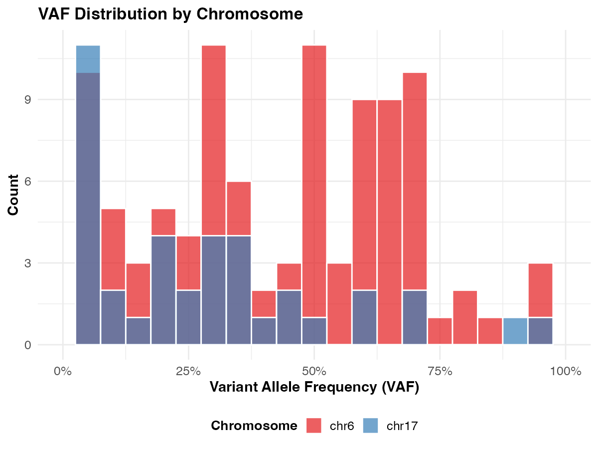

Tip3. VAF density plot

ggplot(vaf_data, aes(x = tumor_af, fill = chr)) +
  geom_density(alpha = 0.5) +
  geom_vline(xintercept = 0.5, linetype = "dashed", color = "grey40") +
  annotate("text", x = 0.52, y = Inf, label = "Expected clonal\nheterozygous",
           hjust = 0, vjust = 1.5, size = 3.5, color = "grey40") +
  labs(
    title = "VAF Density Distribution",
    x = "Variant Allele Frequency (VAF)",
    y = "Density",
    fill = "Chromosome"
  ) +
  scale_x_continuous(labels = scales::percent_format(), limits = c(0, 1)) +
  scale_fill_brewer(palette = "Set1") +
  theme_course()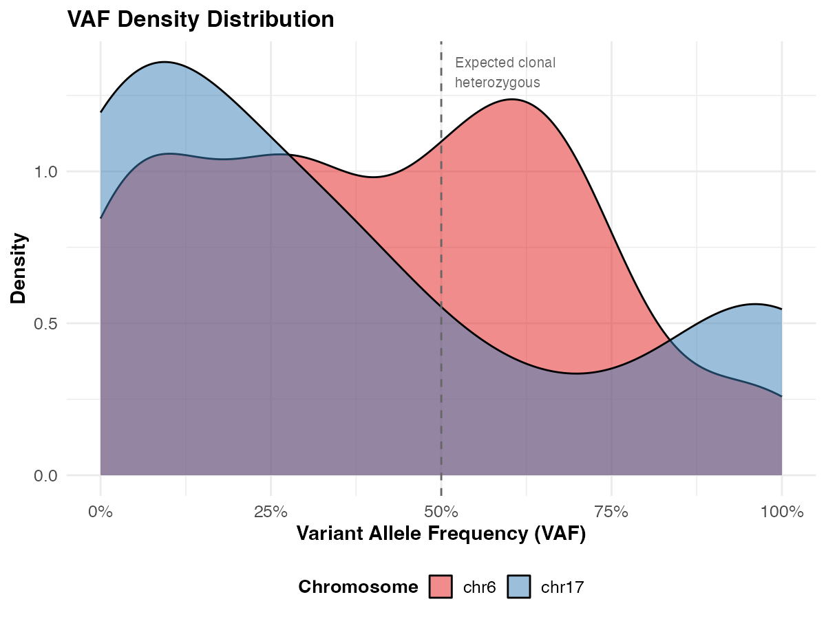

The dashed line at 50% marks the expected VAF for a clonal heterozygous variant in a pure tumor sample. Peaks below this suggest either subclonal variants, lower tumor purity, or copy number alterations — all concepts covered in the Day 2 lecture.

Interpretation guide

VAF range	Likely interpretation
~50%	Clonal heterozygous variant in pure tumor
~25%	Clonal het variant at ~50% purity, or subclonal at high purity
<10%	Subclonal variant, low purity, or sequencing artifact
~100%	Homozygous variant or loss of heterozygosity (LOH)

NoteConnecting VAF to the AMP/ASCO/CAP framework

VAF alone doesn’t determine clinical tier, but it informs interpretation:

• High VAF clonal variants in known cancer genes are more likely to be drivers
• Low VAF variants may represent subclonal populations or early mutations in tumor evolution
• Comparing tumor vs normal VAF (which Mutect2 does internally) distinguishes somatic from germline